A Practical Guide to Building Recommender Systems with NMF and Latent Factors

In modern digital content platforms, many systems rely on techniques like Non-Negative Matrix Factorization (NMF) to power their recommendations. At the same time, users are often overwhelmed by a large number of choices. Consequently, most people now prefer scrolling through recommended lists. Instead of actively searching for new content, they simply pick something that catches their eye. As a result, the quality of these recommendations plays a key role in shaping the user experience on the platform.

Because of this shift, recommendation systems have become the backbone of many digital products. In practice, in video streaming services and e-commerce platforms, suggesting the right content at the right time not only improves user experience. Furthermore, it directly boosts key business metrics like retention and engagement.

In this post, we will look at the movie recommendation problem from a technical point of view, focusing on Non-Negative Matrix Factorization (NMF). This is a method based on latent factors that is both effective and easy to understand. In particular,  it will show how NMF helps understand user preferences from sparse data and how it can be used in practice to build recommendation systems.

The “What Movie Should I Watch Tonight?” Problem: NMF and Sparse Matrices

In many modern digital platforms, from movie streaming apps to e-commerce marketplaces, the core question is always the same:

How do we suggest the right item to a user from thousands of available options?

To address this, recommendation systems typically start with user behavior data. Therefore, the data is represented in a common structure known as the User-Item Matrix.

1. Context: Representing Movie Preferences in a User-Item Matrix

To make this more concrete, let’s assume our system has access to a database of movie ratings. To allow the system to learn user preferences, this data is represented as a large matrix:

• Rows represent individual users.
• Columns represent movies in the library.
• Each cell contains a rating (e.g., 1 to 5 stars) that a user has given to a movie.

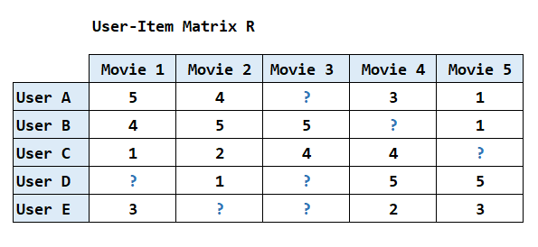
Table 1: The User-Item Matrix structure, where rows are users and columns are movies.

From a practical perspective, this matrix acts as a "preference map,". Moreover, it enables the system to see the relationships between users and the content they have interacted with. In addition, it serves as the foundation for most modern Collaborative Filtering approaches. However, this representation quickly reveals a fundamental limitation.

2. The Problem: The Paradox of the Sparse Matrix

However, when we take a closer look at the User-Item Matrix, a major issue becomes clear: most of the cells are empty.

In reality, even the most active users only watch and rate a small fraction of the thousands of movies available. In practice, the percentage of cells containing actual rating data is often less than 1%.

As a result, we are dealing with a sparse matrix. Because the amount of observable information is very limited, traditional methods often fail to compare users or movies effectively.

3. The Challenge: Predicting from the Gaps

The extreme sparsity of the data creates the core challenge for recommendation systems:

How do we accurately predict ratings for movies that users have never seen?

If the system can predict that a user will enjoy a thriller movie they’ve never heard of, we have a basis to prioritize that title in their recommendations. However, the goal here is not just to fill in the blanks with random numbers. Instead, we want to discover the hidden relationships that drive user behavior, such as favorite genres, storytelling styles, or aesthetic tastes.

At this point, Non-negative Matrix Factorization (NMF) becomes an effective approach. It helps extract hidden features from a sparse rating matrix, providing a foundation for building meaningful and easy-to-interpret recommendations. At this stage, we need a model that can learn meaningful patterns from incomplete data.

The way NMF looks at movie ratings

To solve the sparse matrix problem, Non-negative Matrix Factorization (NMF) uses a mathematical technique to uncover the hidden factors behind each user rating. Instead of just looking at numbers, NMF attempts to answer a key question: Why does a user like or dislike a movie?

In the world of NMF, we don't just see a "4 star rating." Instead, the algorithm assumes that every rating is the result of several hidden features. For example, a user might like a movie because it is a "Sci-fi" film with "High Action" and a "Fast Pace." By breaking the large matrix into smaller parts, NMF helps us identify these hidden patterns.

1. Decomposition Mechanism: Divide to Understand

NMF factorizes the original rating matrix R into the product of two smaller matrices, W and H:

• The User Matrix (W): This matrix represents user preference profiles. Each row shows how much a user is interested in different "movie vibes," such as action, romance, or mystery.
• The Movie Matrix (H): This matrix describes the characteristics of each movie. Each column represents a movie as a combination of hidden features, each with its own weight.

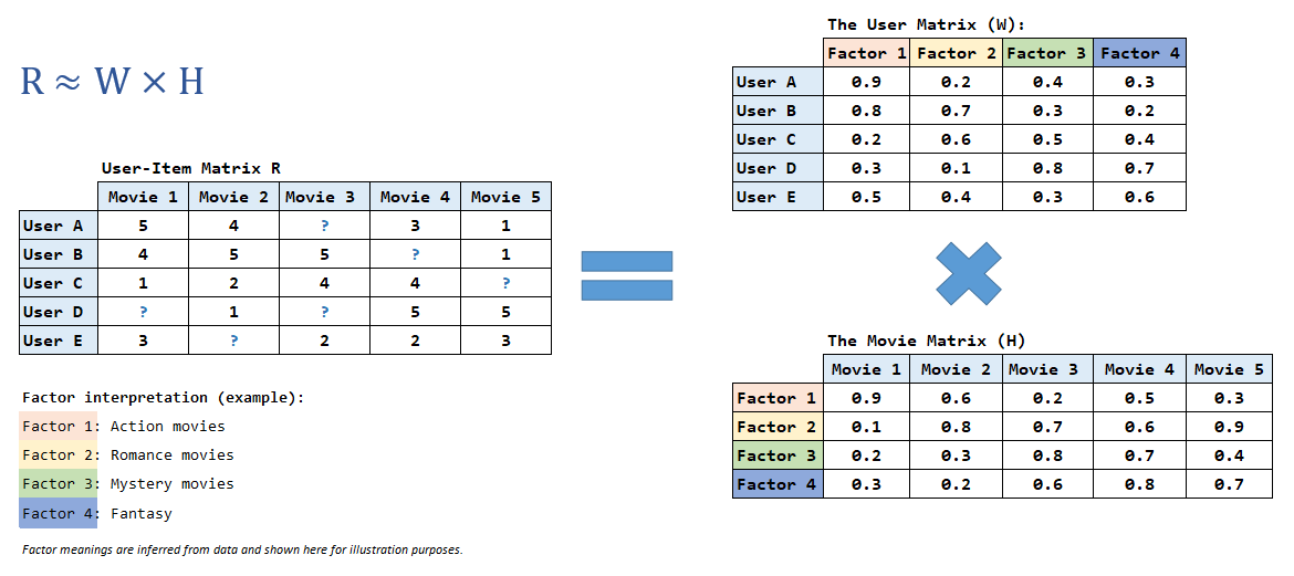
From an intuitive perspective, the system does not store thousands of empty cells. Instead, it learns compact representations of both users and movies using a small number of hidden features. By connecting these two matrices, the system can fill in the missing ratings and provide meaningful recommendations.

2. The Additive Property: Why NMF Is Easy to Explain

A key idea behind NMF is that all values in its matrices are non-negative. This means each recommendation is built by adding together positive factors, rather than mixing positive and negative signals.

For example, when a user likes a Marvel movie such as The Avengers, NMF can explain this preference as a combination of factors:

Score = Superheroes + Action + Visual Effects

Because there are no negative values, these factors simply add up to form the final score instead of canceling each other out. Consequently, this additive nature makes NMF especially easy to interpret. It helps data engineers clearly explain to other teams why a specific movie was recommended.

3. Why This Approach Works

By doing so, when we multiply matrices W and H back together, we get a predicted rating matrix. In this new matrix, the empty cells from the original data are filled with estimated values.

In fact, these values are not random. Instead, they are the result of combining a user’s specific preferences with the actual characteristics of the movies. In this way, NMF allows the system to "see" movies in a way that is much closer to human intuition. By predicting these missing scores, we can identify which movies a user is most likely to enjoy, even if they have never interacted with them before. With this intuition in mind, we can now move on to the practical implementation.

NMF Implementation Steps

Step 1: Environment Setup and Data Exploration for NMF (EDA)

Before building the NMF model, we first need to prepare the environment and create a dataset that simulates a real-world movie recommendation scenario.

1.1. Installing Required Libraries

For this project, we will use the most common Python libraries in the data science ecosystem:

py -m pip install numpy pandas scikit-learn

1.2. Creating a Synthetic Rating Dataset

Instead of using public datasets, we will create a synthetic dataset to mimic real-world user-movie interactions. This allows us to better control the environment and demonstrate the challenge of data sparsity.

Our Dataset Assumptions:

• 1,000 users and 1,000 movies.
• Each user rates approximately 25 movies on average.

import numpy as np
import pandas as pd

# For reproducibility
np.random.seed(42)

num_users = 1000
num_movies = 1000
ratings_per_user = 25

data = []
for user_id in range(num_users):
    # Each user randomly picks 25 unique movies
    movie_ids = np.random.choice(
        num_movies, ratings_per_user, replace=False
    )
    # Assign a random rating from 1 to 5
    ratings = np.random.randint(1, 6, size=ratings_per_user)

    for movie_id, rating in zip(movie_ids, ratings):
        data.append([user_id, movie_id, rating])

# Create the DataFrame
ratings_df = pd.DataFrame(
    data, columns=["user_id", "movie_id", "rating"]
)

print(ratings_df.head())

This dataset reflects a common real-world pattern. Each user interacts with only a small fraction of the available content. In this case, only 2.5% of the matrix contains ratings.

1.3. Building the User-Item Rating Matrix R

Next, we convert our tabular data into a User-Item Matrix (R). In practice, this is the standard input format for NMF.

# Convert the DataFrame into a pivot table
R = ratings_df.pivot(
    index="user_id",
    columns="movie_id",
    values="rating"
).fillna(0)

print(f"Matrix shape: {R.shape}")

Key details about Matrix R:

• Rows represent individual users.
• Columns represent movies in the library.
• A value of 0 indicates a missing rating (the user has not watched or rated that movie yet).

In this example, the matrix shape is (1000, 1000), meaning we have a grid of 1 million possible interactions, though most of them are currently zero.

1.4. Measuring Matrix Sparsity

Before moving to the model, we need to measure the Sparsity of our dataset. This metric tells us exactly how much information is missing.

# Count the number of actual ratings
num_ratings = np.count_nonzero(R.values)
total_cells = R.size  # Total number of user-movie pairs

# Calculate the percentage of empty cells
sparsity = 1 - (num_ratings / total_cells)
print(f"Sparsity: {sparsity:.2%}")

Example output: Sparsity: 97.50%

This result gives us two important insights:

• First, only 2.5% of all possible user-movie pairs contain actual ratings.
• Meanwhile, the remaining 97.5% of the matrix consists of missing values that the system needs to predict.

Therefore,  high sparsity is a common challenge in real-world systems, and it is exactly why we need a powerful technique like NMF to fill in the gaps.

1.5. Rating Distribution Analysis

Finally, we examine the distribution of rating values to understand how users typically rate movies in our dataset.

# Check the frequency of each rating value
rating_counts = ratings_df["rating"].value_counts().sort_index()
print(rating_counts)

Example output:

rating
1    4939
2    4985
3    4947
4    5052
5    5077

Key Observations:

• Even Distribution: Ratings are relatively evenly distributed from 1 to 5.
• No Strong Bias: There is no extreme bias toward only high (e.g., all 5s) or only low (e.g., all 1s) ratings.
• Model Readiness: This balanced dataset is ideal for applying NMF because it provides a diverse range of feedback for the algorithm to learn from.

Step 2: Building the NMF Model with Python

After preparing the data and constructing our rating matrix R, we are ready to train the Non-Negative Matrix Factorization (NMF) model. Our goal is to extract the hidden factors that explain the ratings in our dataset.

2.1. Importing the Library

For this implementation, we will use the NMF class provided by scikit-learn. This implementation is stable and widely used for practical recommender system applications.

from sklearn.decomposition import NMF

2.2. Choosing the Number of Latent Factors (k)

One of the most important hyperparameters in NMF is the number of latent factors, denoted as k. This value determines how many "hidden features" the model will use to explain user preferences.

For this example, we will set: n_components = 15

What does k = 15 mean?

• Learning "Vibes": The model attempts to learn 15 distinct "movie vibes" from the data.
• Auto discovery: These factors are not predefined categories (like "Action" or "Comedy"). Instead, they are patterns discovered automatically by the algorithm from user ratings.
• Balanced Complexity: A value of k=15 is a reasonable choice for this demo. It is large enough to capture major preference patterns, but small enough to keep the model fast and simple.

2.3. Initializing and Training the Model

Now, we initialize the NMF model and fit it to our rating matrix R.

# Initialize NMF with 15 latent factors
nmf = NMF(
    n_components=15,
    init="nndsvd",   # Recommended for sparse data
    random_state=42,
    max_iter=800
)

# Decompose the matrix R into W and H
W = nmf.fit_transform(R)
H = nmf.components_

Understanding the Output:

• The W Matrix (User-Feature): This represents how strongly each user is associated with each of the 15 latent factors. You can think of this as a "User Profile" based on their tastes.
• The H Matrix (Feature-Movie): This describes how each movie is composed of those same 15 factors. It acts as a "Movie Profile" that defines its characteristics.

Why use init="nndsvd"?

• This initialization method is highly effective for sparse datasets. It helps the model converge faster and stay more stable during training, ensuring that we get reliable results even with limited data.

2.4. Quick Sanity Check

To verify that the model has been trained correctly, we should check the shapes of our new matrices. This ensures that the decomposition process has followed our defined parameters.

# Check the dimensions of the output matrices
print(f"Shape of W (Users): {W.shape}")
print(f"Shape of H (Movies): {H.shape}")

Output:

(1000, 15)
(15, 1000)

What does this confirm?

• User Representation: Our 1,000 users are now represented in a 15-dimensional latent space. Instead of 1,000 movie ratings, each user is now described by just 15 core preferences.
• Movie Mapping: Similarly, our 1,000 movies are mapped into the same latent feature space. Each movie is now defined by how much it aligns with those 15 hidden characteristics.

Step 3: Interpreting the Latent Factors

One of the biggest advantages of Non-Negative Matrix Factorization (NMF) is that its latent factors are often easy to interpret. Instead of treating the model as a "black box," we can inspect what each factor actually represents.

3.1. Inspecting the Movie–Latent Feature Matrix (H)

After training, we obtain the matrix H, where:

• Row corresponds to a latent factor.
• Column corresponds to a movie.
• Value shows how strongly a movie is associated with that specific factor.

Therefore, in practice, we interpret a latent factor by looking at the movies that have the highest weights for it.

3.2. Finding the Top Movies for Each Factor

The following code extracts the top movies for a specific latent factor:

def get_top_movies_for_factor(H, factor_id, top_n=10):
    # Sort indices by weight in descending order
    top_movie_indices = np.argsort(H[factor_id])[::-1][:top_n]
    return top_movie_indices

# Example: Inspecting Factor #5
factor_id = 5
top_movies = get_top_movies_for_factor(H, factor_id)
print(f"Top movie indices for Factor #{factor_id}: {top_movies}")

Output:

Top movie indices for Factor #5: [973 371 334 517 883 502 889 157 383  29]

3.3. How to Interpret the Results

Suppose the top movies for Factor #5 are:

• Toy Story
• Shrek
• Finding Nemo
• Monsters

From this list, we can clearly see that a common pattern emerges.

Rather than being a predefined genre, Factor #5 appears to capture a shared theme:

animated, family-friendly movies

We can therefore interpret Factor #5 as something like:

“Family Animation”

This label is inferred by us (the humans), but the fact that the model consistently groups similar movies together is a key strength of NMF.

3.4. Why This Matters?

This interpretability is what sets NMF apart from many black-box models:

• We do not just know what the model recommends
• We also understand why a recommendation was made

For example, instead of saying:

“This movie was recommended because the model says so”

We can say:

“This movie was recommended because it aligns strongly with the user’s preference for animated, family-oriented films”

This makes NMF especially attractive in scenarios where:

• Explaining recommendations to non-technical stakeholders (like Product or Marketing teams).
• Building trust with users by providing clear reasons for suggestions.
• Debugging the model to see if it is learning meaningful patterns.

Step 4: Recommending Movies for a Specific User

With our trained matrices W and H, we can now generate personalized movie recommendations. As a result, the model’s “learning” turns into actual user value.

4.1. Predicting Ratings for Unseen Movies

First, we select a user from our dataset. For example, let’s look at User #42. The corresponding row in matrix W represents this user’s preference profile across our 15 latent factors.

Next, to estimate how much this user would enjoy each movie in the library, we compute the dot product between the following two components:

• The user’s preference vector (from W)
  The movie feature matrix (H)

# Get the preference vector for User 42
user_vector = W[user_id]

# Calculate predicted ratings for all 1,000 movies
predicted_ratings = np.dot(user_vector, H)

4.2. Filtering Already Seen Movies

A good recommendation system shouldn't suggest movies the user has already watched. We filter these out by looking at the original matrix R:

# Identify movies the user has already rated
already_rated = R.iloc[user_id] > 0

# Set their predicted scores to -1 so they aren't recommended
predicted_ratings[already_rated.values] = -1

4.3. Generating Top-N Recommendations

Finally, we select the top 5 movies with the highest predicted scores:

top_n = 5
recommended_movie_ids = np.argsort(predicted_ratings)[::-1][:top_n]

print(f"Top 5 Recommendations for User {user_id}: {recommended_movie_ids}")

Output:

Top 5 Recommendations for User 999: [225 934 359 265 736]

Evaluation and Limitations

In this final section, we briefly discuss how to evaluate the model's performance and address some of the inherent limitations of this approach. From an evaluation standpoint, it is important to quantify how well the model performs.

1. Evaluation Metric

In practice, Root Mean Square Error (RMSE) is commonly used to evaluate recommendation systems. It measures how closely our predicted ratings match the actual ratings given by users. A lower RMSE indicates that our model is better at "guessing" user preferences based on the known interactions. Next, we need to consider how model complexity affects both performance and interpretability.

2. Selecting the Best k

Choosing the number of latent factors (k) is a balancing act. If k is too small, the model might miss important details. On the other hand, if k is too large, the model might become over-complicated.
In real-world projects, k is typically selected using:

• The Elbow Method: Visualizing where the error starts to level off.
• Cross-validation: Testing the model on a hidden portion of the data to ensure it generalizes well.

3. NMF Limitations

Despite its strengths, NMF is a collaborative filtering method, which means it relies heavily on past interactions. This leads to the "Cold Start" problem:

• New Users: Without a history of ratings, the model cannot effectively build a preference profile.
• New Movies: Items without any ratings cannot be recommended because the model hasn't "learned" their features yet.

As a result, many real-world systems extend NMF with additional techniques. To solve these issues, modern systems often use Hybrid Approaches, combining NMF with content-based filtering (using movie metadata like actors, directors, or descriptions) to ensure everyone gets great recommendations from day one.

Conclusion

In conclusion, we have explored how to build a movie recommendation system using Non-Negative Matrix Factorization (NMF). Taken together, this approach provides a clear and practical way to handle sparse data. We covered everything from handling sparse data to generating personalized suggestions.

More importantly, several key lessons stand out from this approach.:

• NMF is easy to explain: Unlike black-box models, NMF helps us understand why a movie is recommended by looking at shared themes and hidden factors.
• Built for trust: Because it is easy to interpret, NMF is a great choice for systems where transparency matters, helping both users and stakeholders trust the results.
• Great for sparse data: NMF provides a perfect balance of simplicity and effectiveness, making it a reliable starting point for any recommendation project.

For these reasons, NMF remains a strong baseline method for many real-world recommendation systems.

References

1. Scikit-learn Documentation (NMF): https://scikit-learn.org/stable/modules/generated/sklearn.decomposition.NMF.html
2. Algorithms for Non-negative Matrix Factorization: proceedings.neurips.cc/paper_files/paper/2000/file/f9d1152547c0bde01830b7e8bd60024c-Paper.pdf
3. Nonnegative Matrix Factorization for Dummies: https://www.billconnelly.net/?p=534
4. Featured Image: https://www.pexels.com/photo/a-laptop-screen-with-text-4439901/