In PCA image classification tasks, the input data is often high-dimensional, containing a large number of features. For example, a 64×64 RGB image consists of 3 color channels, resulting in 64 × 64 × 3 = 12,288 numerical pixel values. When we feed all 12,288 raw pixel values directly into traditional machine learning models, several issues typically arise:
-
-
- Slow processing speed
- Difficulty learning the important features
-
- High sensitivity to noise
- Increased risk of overfitting
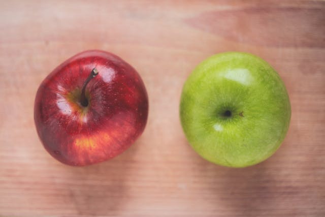
Principal Component Analysis (PCA) is a dimensionality-reduction technique that preserves the most important information in the data while reducing noise. To illustrate how PCA works in practice, this article uses a clear and intuitive example: distinguishing between green apples and red apples using Scikit-learn - a simple task that effectively demonstrates the benefits of PCA in image classification.

1. What is Principal Component Analysis (PCA)?
Principal Component Analysis (PCA) is a statistical method that helps to:
- Identify the directions where the data varies the most (the principal components)
- Transform the data into a new coordinate system
- Retain the most important components
- Reduce the dimensionality while preserving the main structure of the information
To understand this concept clearly, we first need to explain what a “dimension” is in image data.
Understanding “Dimension” in Image Data
In machine learning, each feature in the data is considered one dimension.
- A data table with 3 columns corresponds to 3 dimensions.
- A vector with 10 values represents 10 dimensions.
When applied to images:
- A 64×64 RGB image contains 3 color channels, resulting in 12,288 numerical pixel values.
- Each pixel represents a light–dark value, making it a feature.
- The entire image can be represented as a 12,288-dimensional vector.
We can say that a “dimension” is the number of independent pieces of information the model must handle. Because an image has thousands of pixels, it also has thousands of dimensions, meaning the model must process a large amount of highly varied information.
How Does PCA Work?
PCA has two main purposes:
- First, it identifies the directions in an image where the data varies the most — these are known as the principal components.
- Second, by keeping only these high-variance components and discarding low-variance information (often noise), the method effectively reduces the dimensionality of the data.
Applying PCA to the green–red apple example:
- High-variance regions such as the apple’s contour, stem area, and strong color differences between green and red are preserved.
- Low-variance regions such as uniform background, shadows, or noise on the table surface are filtered out.
As a result, the original 12,288-dimensional RGB image can be compressed to around 100 dimensions, while still keeping the core information needed for the model to classify the image.
2. Why Is PCA Important in Image Classification?
2.1. Image is High-dimensional
In our example, a 64×64 RGB image corresponds to 12,288 numerical pixel values, which means it has 12,288 dimensions. In traditional machine learning models, this leads to several problems:
- Slow processing speed
- Difficult optimization
- Difficulty separating cats from dogs
⇒ PCA reduces the number of dimensions to around 100, helping the model learn faster and with greater stability.
2.2. Many Pixels Are Irrelevant to Classification
For example:
- Wall background
- Uniform dark regions
- Grass
- Details that are far from the main object
⇒ These regions do not help distinguish between green apples and red apples, so PCA automatically reduces their influence.
2.3. PCA Highlights the Important Features
Thanks to PCA, the model focuses on:
-
- Overall apple shape
-
- Strong color differences between green and red regions
- Surface texture patterns
- Brightness and shading variations on the peel
- Stem area and contour lines
- Local color gradients unique to each apple type
These are the features that truly help the model classify the image.
2.4. Improve the Performance of Traditional Models
Models such as Logistic Regression (LR), Support Vector Machine (SVM), and Random Forest cannot efficiently handle images with 12,288 dimensions.
PCA transforms the images into a new feature space, allowing these models to:
- Separate the classes more easily: PCA creates a new feature space where green and red apple images become “farther apart” in a mathematical sense (distance/variance). When the two classes are farther apart, the classifier can draw the decision boundary much more easily.
- Generalize better: By removing noise and redundant information, the model focuses only on meaningful features.
- Achieve higher accuracy: Since the input becomes cleaner and more compact, the classifier makes more reliable predictions.
3. Using Scikit-learn to Illustrate PCA in Image Classification
3.1. Preparing the environment and libraries
py -m pip install numpy pillow scikit-learn3.2. Data normalization
This step is part of the preprocessing stage, where raw images are normalized and converted into a numerical format suitable for PCA and machine learning models.
# dataset_loader.py
import os
import numpy as np # Handle matric, flatten
from PIL import Image # Open images, convert to RGB, resize
def load_images(folder, label):
    """
    1. Load images from a given folder
    2. Convert them to RGB (keep color information),
    3. Resize them to 64×64
    4. Normalize to [0, 1] and flatten to 1D vectors (64×64×3 = 12,288 dimensions),
    5. Return both the processed images and their corresponding labels (0 for green_apple, 1 for red_apple).
    Parameters
    ----------
    folder : str
        Path to the folder containing the images.
    label : int
        The numerical label assigned to all images in this folder
        (0 for green_apple, 1 for red_apple).
    Returns
    -------
    images : numpy.ndarray
        Array of shape (N, 12288), where N is the number of images.
        Each row represents one flattened RGB image.
    labels : numpy.ndarray
        Array of shape (N,), containing the label for each image.
    """

    images, labels = [], []
    # Iterate through all files in the folder
    for filename in os.listdir(folder):
        if filename.startswith("."):
            continue
        if not filename.lower().endswith((".jpg", ".jpeg", ".png", ".bmp")):
            continue
        path = os.path.join(folder, filename)
        # Open the image, convert to RGB, and resize to 64×64
        img = Image.open(path).convert("RGB").resize((64, 64))
        # Convert to float32 NumPy array in [0, 1] and flatten
        arr = np.array(img, dtype=np.float32) / 255.0
        images.append(arr.flatten())
        # Append the label for this image
        labels.append(label)
    # Return as NumPy arrays for compatibility with ML models
    return np.array(images), np.array(labels)
3.3. Dimensionality Reduction with PCA
# pca_reduction.py
import numpy as np
from sklearn.decomposition import PCA
from sklearn.preprocessing import StandardScaler
from dataset_loader import load_images

def run_pca():
    """
    Load green_apple and red_apple images, combine them into a single RGB dataset,
    apply PCA to reduce dimensionality from 12,288 to configurable components,
    and return the transformed data along with their labels and the PCA model.

    Returns
    -------
    X_pca : numpy.ndarray
        PCA-transformed feature matrix.
    y : numpy.ndarray
        Label array for all images (0 = green_apple, 1 = red_apple).
    pca : sklearn.decomposition.PCA
        The trained PCA transformer.
    scaler : sklearn.preprocessing.StandardScaler
        Fitted scaler from training step.
    feature_scaler : sklearn.preprocessing.StandardScaler
        Scaler applied after PCA to keep features well conditioned.
    """

    # Load preprocessed green_apple images (label = 0)
    X_green_apples, y_green_apples = load_images("dataset/green_apples", label=0) # Images of green_apple
    # Load preprocessed red_apple images (label = 1)
    X_red_apples, y_red_apples = load_images("dataset/red_apples", label=1) # Images of red_apple

    # Combine green_apple + red_apple feature matrices into one dataset
    X = np.vstack([X_green_apples, X_red_apples])
    y = np.hstack([y_green_apples, y_red_apples])

    # Scale before PCA
    scaler = StandardScaler(with_mean=True, with_std=False)
    X_scaled = scaler.fit_transform(X)
    X_scaled = X_scaled.astype(np.float64, copy=False)

    # Create PCA with configurable number of components
    pca = PCA(
        n_components=100,
        random_state=42,
        svd_solver="full",
        whiten=False,
    )

    # Fit PCA on X and transform it
    X_pca = pca.fit_transform(X_scaled)


    # Scale PCA features to keep them well conditioned for linear models
    feature_scaler = StandardScaler()
    X_pca_scaled = feature_scaler.fit_transform(X_pca)

    print("Original shape:", X.shape)
    print("After PCA:", X_pca.shape)

    return X_pca_scaled, y, pca, scaler, feature_scaler
At this point, the dimensionality reduction step is complete. The original 12,288-dimensional RGB images have been compressed into just 100 dimensions. X_pca now represents the transformed dataset — more compact, cleaner, and easier for the model to learn from.
3.4. Training a Classifier on PCA Features (Logistic Regression)
# classification.py
import numpy as np
from sklearn.linear_model import LogisticRegressionCV
from sklearn.metrics import accuracy_score
from sklearn.model_selection import StratifiedKFold, train_test_split
from pca_reduction import run_pca
def train_model():
    """
    Train a logistic regression model on PCA reduced features.
    Returns
    -------
    model : sklearn.linear_model.LogisticRegressionCV
        Trained classifier.
    pca : sklearn.decomposition.PCA
        Fitted PCA transformer.
    scaler : sklearn.preprocessing.StandardScaler
        Fitted scaler.
    feature_scaler : sklearn.preprocessing.StandardScaler
        Scaler applied after PCA so inference matches training.
    metrics : dict
        Dictionary containing evaluation metadata.
    """
    X_pca, y, pca, scaler, feature_scaler = run_pca()
    # Split the PCA features and labels into train (80%) and test sets (20%)
    X_train, X_test, y_train, y_test = train_test_split(
        X_pca, y, test_size=0.2, stratify=y, random_state=42
    )
    # Cross-validated logistic regression improves generalization accuracy
    cv = StratifiedKFold(n_splits=5, shuffle=True, random_state=42)
    model = LogisticRegressionCV(
        Cs=np.logspace(-2, 2, 9),
        cv=cv,
        max_iter=2000,
        scoring="accuracy",
        n_jobs=1,
        refit=True,
        solver="liblinear",
    )

    # Train the model on the PCA-transformed training data
    model.fit(X_train, y_train)
    # Predict labels for the test set
    y_pred = model.predict(X_test)
    # Compute classification accuracy
    acc = accuracy_score(y_test, y_pred)
    metrics = {
        "test_accuracy": acc,
        "train_size": len(X_train),
        "test_size": len(X_test),
        "best_C": float(model.C_[0]),
    }
    print(
        f"Test accuracy: {acc:.4f} "
        f"(train={len(X_train)} samples, test={len(X_test)} samples, best C={model.C_[0]:.4f})"
    )
    return model, pca, scaler, feature_scaler, metrics
3.5. Predict a new image
# predict.py
import os
import numpy as np
from PIL import Image
from classification import train_model
LABEL_TO_NAME = {0: "Green", 1: "Red"}
def prepare_image(path):
    img = Image.open(path).convert("RGB").resize((64, 64))
    arr = np.array(img, dtype=np.float32) / 255.0
    return arr.flatten().reshape(1, -1)
def predict_image(path, pca, scaler, feature_scaler, model):
    img_vec = prepare_image(path)
    # Apply the same scaling used during training
    img_scaled = scaler.transform(img_vec).astype(np.float64, copy=False)
    # Apply PCA transform
    img_pca = pca.transform(img_scaled)
    # Scale PCA features to keep them well conditioned for linear models
    img_pca_scaled = feature_scaler.transform(img_pca)
    # Predict label
    pred = model.predict(img_pca_scaled)[0]
    return LABEL_TO_NAME.get(pred, "Unknown")
def predict_folder(folder_path, pca, scaler, feature_scaler, model):
    print(f"Testing folder: {folder_path}")
    y_true, y_pred = [], []
    for file in os.listdir(folder_path):
        if file.startswith("."):
            continue
        if not file.lower().endswith((".jpg", ".jpeg", ".png", ".bmp")):
            continue
        path = os.path.join(folder_path, file)
        label_name = predict_image(path, pca, scaler, feature_scaler, model)
        print(f"{file} ➝ {label_name}")
def main():
    model, pca, scaler, feature_scaler, metrics = train_model()
    print(f"Training metrics: {metrics}")
    predict_folder(
        "dataset/test_apples",
        pca,
        scaler,
        feature_scaler,
        model
    )
if __name__ == "__main__":
    main()
After running the model on several test images, we obtain the predictions shown below:
green_01.jpg ➝ Green
green_02.jpg ➝ Green
green_03.jpg ➝ Green
green_04.jpg ➝ Green
green_05.jpg ➝ Red
red_01.jpg ➝ Green
red_02.jpg ➝ Red
red_03.jpg ➝ Green
red_04.jpg ➝ Red
red_05.jpg ➝ Red
The filenames were assigned according to the true color of each apple (“green” for green apples and “red” for red apples). As shown, most predictions match the ground truth, while a few images were misclassified—likely due to lighting, shadows, or color overlap between the two varieties. This demonstrates both the effectiveness of PCA & Logistic Regression and the natural challenges of real-world image data.
4. Conclusion
Through the example of classifying green apples and red apples, we can clearly see that Principal Component Analysis:
- Significantly reduces the dimensionality of RGB images
- Effectively removes noise and irrelevant information
- Highlights the most important visual features such as color and shape
- Accelerates model training
- Improves the accuracy and stability of traditional machine learning models
PCA remains one of the foundational techniques in image processing and classical machine learning, especially valuable when resources are limited or when the pipeline does not rely on deep learning.
References
1. Principal Component Analysis (PCA): https://www.geeksforgeeks.org/data-analysis/principal-component-analysis-pca/
2. scikit-learn API Reference: Principal component analysis (PCA): https://scikit-learn.org/stable/modules/generated/sklearn.decomposition.PCA.html
3. scikit-learn API Reference: Logistic Regression CV: https://scikit-learn.org/stable/modules/generated/sklearn.linear_model.LogisticRegressionCV.html
4. Featured Image: https://www.pexels.com/photo/robot-pointing-on-a-wall-8386440/
5. Example Image: https://www.pexels.com/photo/two-red-and-green-apple-fruits-on-brown-surface-135130/


